Olympia oyster epigenetics
For primer 2 samples analysis = primer 2 ETS, panel = primer 2 0325, size standard = GS500 040113. No samples failed size standard. Genotyped all primer 2 samples and began analysis of primer 3 - edited analysis method as described 6/12/13 and ran analysis of samples. The samples include those also run 3/25/13. No samples for primer 3 failed size standard. Got through sample DAB093_Msp3 for adding and editing bins.
June 19, 2013
Olympia oyster epigenetics
Select PCR using primer pairs 2, 3, 4. Meant to finish primer set 2, but accidentally used preselect PCR Msp template for the first 2 columns of the plate instead of Hpa (not a huge deal since I need to re-PCR some individuals to get error rate at some point anyway). PCR'd all samples for primer set 3, and first 16 for primer set 4. There wasn't quite enough AmpliTaq Gold left for 4, so those PCRs might be weak/not work. Used program PRESEL on thermalcycler.
Accidentally made too much master mix so there is a tube containing enough mix for 32 reactions (without taq or primers, amplitaq gold buffer was used).
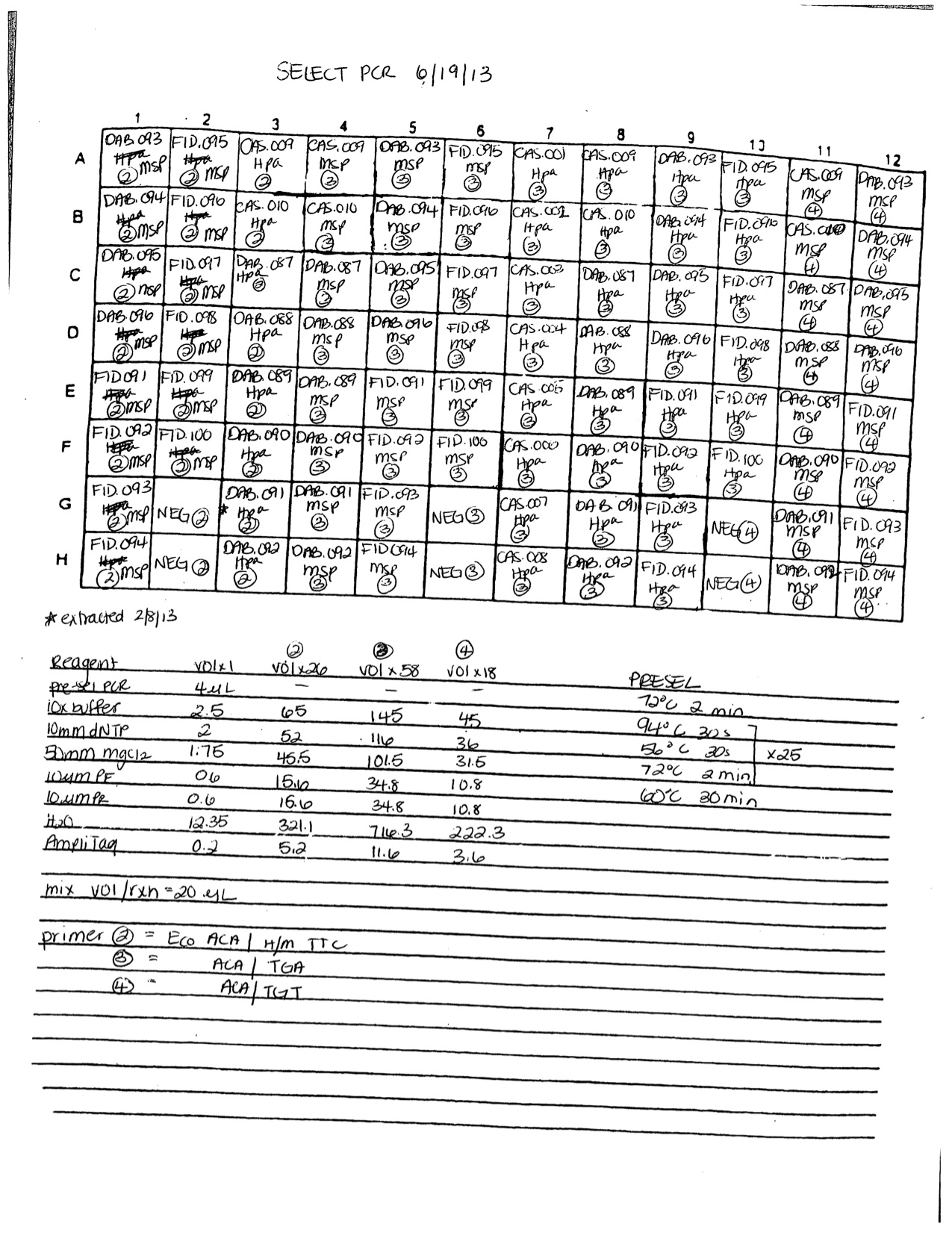
Diluted the PCR in milliQ water (1:15, except for the last 2 columns - primer set 4 - which were diluted 1:10). Mixed 10 µl ROX 500 with 1490 µl formamide and aliquoted 15 µl to a new welled plate. Added 1 µl of diluted PCR product to the formamide/ROX. Ran on ABI 3730.
June 13, 2013
Olympia oyster epigenetics
With all the primer 1 data in one spreadsheet, I grouped all the common alleles together so that they are in the same column for each sample. The total number of MSAFLP alleles is 125, ranging from 56-533 bp. Removed samples from dataset if they did not have data for both restriction enzymes (CAS007, CAS008, FID 093).
In SQLshare changed allele values to presence/absence (1/0) indicators using the following code:
SELECT Allele1, Allele2,...Allele125,
CASE WHEN Allele1>0 then 1 ELSE 0 END
AS Al1,
CASE WHEN Allele2>0 ELSE 0 END
AS Al2,....
AS AL125
FROM [table_Primer 1 data.txt]
From the binary data, made new columns for methylation status. For each sample, the 1st methylation status (methstat) column indicates whether the locus has the potential to be methylated, i.e. if the fragment is present in both enzyme digests then the sample is unmethylated at that locus, but if it is present in 1 digest or neither it is a potentially methylatable site. The second methstat column indicates if the locus is informative in terms of methylation status. If there is no band (both hpa and msp have a 0 in the column), then is it uninformative, but if one enzyme has a band and the other does not, then it is methylated.
SELECT [CAS001Hpa1], [CAS001Msp1], [CAS001Hpa1]+[CAS001Msp1] AS [CAS001],
[CAS002Hpa1], [CAS002Msp1], [CAS002Hpa1]+[CAS002Msp1] AS [CAS002],
[CAS003Hpa1], [CAS003Msp1], [CAS003Hpa1]+[CAS003Msp1] AS [CAS003],
[CAS004Hpa1], [CAS004Msp1], [CAS004Hpa1]+[CAS004Msp1] AS [CAS004],
[CAS005Hpa1], [CAS005Msp1], [CAS005Hpa1]+[CAS005Msp1] AS [CAS005],
[CAS008Hpa1], [CAS008Msp1], [CAS008Hpa1]+[CAS008Msp1] AS [CAS008],
[CAS009Hpa1], [CAS009Msp1], [CAS009Hpa1]+[CAS009Msp1] AS [CAS009],
[CAS010Hap1], [CAS010Msp1], [CAS010Hap1]+[CAS010Msp1] AS [CAS010],
[DAB087Hpa1], [DAB087Msp1], [DAB087Hpa1]+[DAB087Msp1] AS [DAB087],
[DAB088Hpa1], [DAB088Msp1], [DAB088Hpa1]+[DAB088Msp1] AS [DAB088],
[DAB089Hpa1], [DAB089Msp1], [DAB089Hpa1]+[DAB089Msp1] AS [DAB089],
[DAB090Hpa1], [DAB090Msp1], [DAB090Hpa1]+[DAB090Msp1] AS [DAB090],
[DAB091Hpa1], [DAB091Msp1], [DAB091Hpa1]+[DAB091Msp1] AS [DAB091],
[DAB093Hpa1], [DAB093Msp1], [DAB093Hpa1]+[DAB093Msp1] AS [DAB093],
[DAB095Hpa1], [DAB095Msp1], [DAB095Hpa1]+[DAB095Msp1] AS [DAB095],
[DAB096Hpa1], [DAB096Msp1], [DAB096Hpa1]+[DAB096Msp1] AS [DAB096],
[FID091Hpa1], [FID091Msp1], [FID091Hpa1]+[FID091Msp1] AS [FID091],
[FID092Hpa1], [FID092Msp1], [FID092Hpa1]+[FID092Msp1] AS [FID092],
[FID094Hpa1], [FID094Msp1], [FID094Hpa1]+[FID094Msp1] AS [FID094],
[FID095Hpa1], [FID095Msp1], [FID095Hpa1]+[FID095Msp1] AS [FID095],
[FID096Hpa1], [FID096Msp1], [FID096Hpa1]+[FID096Msp1] AS [FID096],
[FID097Hpa1], [FID097Msp1], [FID097Hpa1]+[FID097Msp1] AS [FID097],
[FID098Hpa1], [FID098Msp1], [FID098Hpa1]+[FID098Msp1] AS [FID098],
[FID099Hpa1], [FID099Msp1], [FID099Hpa1]+[FID099Msp1] AS [FID099],
[FID100Hpa1], [FID100Msp1], [FID100Hpa1]+[FID100Msp1] AS [FID100]
FROM [primer 1 data binary oysters in col.txt]
SELECT CAS001,
CASE WHEN CAS001=2 then 'NM' WHEN CAS001=1 then 'M' else 'U' END
AS CAS001MethStat,
CASE WHEN CAS002=2 then 'NM' WHEN CAS002=1 then 'M' else 'U' END
AS CAS002MethStat,
CASE WHEN CAS003=2 then 'NM' WHEN CAS003=1 then 'M' else 'U' END
AS CAS003MethStat,
CASE WHEN CAS004=2 then 'NM' WHEN CAS004=1 then 'M' else 'U' END
AS CAS004MethStat,
CASE WHEN CAS005=2 then 'NM' WHEN CAS005=1 then 'M' else 'U' END
AS CAS005MethStat,
CASE WHEN CAS008=2 then 'NM' WHEN CAS008=1 then 'M' else 'U' END
AS CAS008MethStat,
CASE WHEN CAS009=2 then 'NM' WHEN CAS009=1 then 'M' else 'U' END
AS CAS009MethStat,
CASE WHEN CAS010=2 then 'NM' WHEN CAS010=1 then 'M' else 'U' END
AS CAS010MethStat,
CASE WHEN DAB087=2 then 'NM' WHEN DAB087=1 then 'M' else 'U' END
AS DAB087MethStat,
CASE WHEN DAB088=2 then 'NM' WHEN DAB088=1 then 'M' else 'U' END
AS DAB088MethStat,
CASE WHEN DAB089=2 then 'NM' WHEN DAB089=1 then 'M' else 'U' END
AS DAB089MethStat,
CASE WHEN DAB090=2 then 'NM' WHEN DAB090=1 then 'M' else 'U' END
AS DAB090MethStat,
CASE WHEN DAB091=2 then 'NM' WHEN DAB091=1 then 'M' else 'U' END
AS DAB091MethStat,
CASE WHEN DAB093=2 then 'NM' WHEN DAB093=1 then 'M' else 'U' END
AS DAB093MethStat,
CASE WHEN DAB095=2 then 'NM' WHEN DAB095=1 then 'M' else 'U' END
AS DAB095MethStat,
CASE WHEN DAB096=2 then 'NM' WHEN DAB096=1 then 'M' else 'U' END
AS DAB096MethStat,
CASE WHEN FID091=2 then 'NM' WHEN FID091=1 then 'M' else 'U' END
AS FID091MethStat,
CASE WHEN FID092=2 then 'NM' WHEN FID092=1 then 'M' else 'U' END
AS FID092MethStat,
CASE WHEN FID094=2 then 'NM' WHEN FID094=1 then 'M' else 'U' END
AS FID094MethStat,
CASE WHEN FID095=2 then 'NM' WHEN FID095=1 then 'M' else 'U' END
AS FID095MethStat,
CASE WHEN FID096=2 then 'NM' WHEN FID096=1 then 'M' else 'U' END
AS FID096MethStat,
CASE WHEN FID097=2 then 'NM' WHEN FID097=1 then 'M' else 'U' END
AS FID097MethStat,
CASE WHEN FID098=2 then 'NM' WHEN FID098=1 then 'M' else 'U' END
AS FID098MethStat,
CASE WHEN FID099=2 then 'NM' WHEN FID099=1 then 'M' else 'U' END
AS FID099MethStat,
CASE WHEN FID100=2 then 'NM' WHEN FID100=1 then 'M' else 'U' END
AS FID100MethStat,
FROM [emmats@washington.edu].[summed presence absence fragment peaks]
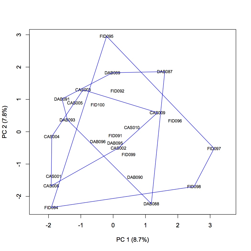
There are between 23-53 methylated loci in each oyster in primer pair 1. A PCA of the data shows no difference in methylation status among sites.
June 12, 2013
Olympia oyster epigenetics
The cut-off criteria for allele calls needs to be more stringent. 3% of max peak height still includes a lot of peaks that are not really peaks. I am adding 2 more filters to choosing peaks: an allele is a true allele if it is at least 10% of the height of the tallest peak (rounded down to the nearest integer); in clusters of adjacent peaks, the tallest is the only allele.
Edited analysis method for primer 1 so that common alleles are not deleted. Also provided cut-off for calling peaks. This only works with "Name alleles using labels". Click Edit labels and enter 400 and 600 as thresholds and 0, Check, 1 as Labels. This will result in no peaks under 400 RFU being called and peaks under 600 will need to be manually checked. Data exported as Primer 1 040113 Genotypes Table2. Repeated for primer 1 data from 3/25/13. Repeated the same steps for primer 2, including the data from 3/25/13 in the 040113 project.
June 11, 2013
Olympia oyster epigenetics
Fragment analysis/epigenotyping of data run 4/2/13 (rerun of run from 4/1, projects are saved as prime 1 040113 and primer 2 040113).
For primer 1: analysis method = primer 1 ETS, panel = primer 1.2, size standard = GS500 040113.
The size standard is bad for samples DAB092_Msp1, DAB094_Msp1, and FID093_Msp1. None of these samples have any data in them so they will have to be rerun. I am deleting them from the project. I have also deleted all of the negative controls and blanks from the project (after ensuring that there was no spurious amplification in any of them).
Project was reanalyzed without the above samples. None of the size quality indicators were red (although about 1/3 are yellow).
For calling peaks, I am going to use the method outlined in Snell-Rood et al. 2013. All potential peaks will be called and then, based on peak heights, quality filtering will be performed outside of GeneMapper. I am still removing allele calls that are obviously not peaks. This means that a peak must have an obvious and clear sharp peak morphology to be called as a MSAFLP allele. Everything >500 bp is also deleted (although none of these resemble true allele peaks).
Added primer 2 samples from run 4/2/13 to project Primer 2 040113. Analysis method = primer 2 ETS, panel = primer 1 0325, size standard =GS500. Edited analysis method so that common alleles are not deleted. A lot of the size standards came back with warnings, so analyzed with GS500 040113 (does not have peaks for 250 or 340). Deleted the following samples from the project since they failed the size standard: CAS008_Msp2, DAB094_Msp2, FID094_Msp2, CAS008_Hpa2. FID093_Msp2 also did not amplify and needs to be redone.
Edited bins so that all allele peaks were included in a bin and saved panel (primer 2 0325). Reanalyzed data.
Exported the genotypes from primer 1 Hpa and Msp. Reformatted the data in Excel so that each allele is a row name and the column headers are individual samples (oysters) - the data in the cells are peak heights for each of the alleles. Checked to see if any called peaks are <3% of the maximum peak height for each sample (none of them were).
June 10, 2013
Secondary stress: transcriptomics
Dan helped me find the problem in my dataset "library reads mapped to isotigs", which is the file with the total mapped reads for each isotig. The numbers that were >999 have quotes around them in the file. I think this is because in Excel the format was set to "general" for the cells. I changed it to "number" and re-uploaded the file, redoing the last query from 6/7/13.
For some of the CGIDs, there are more than 1 matching isotig. Total reads for isotigs were summed within corresponding CGIDs.
SELECT CGID
,sum([EM2A])
,sum([EM2B])
,sum([EM2C])
,sum([EM2D])
,sum([EM2E])
,sum([EM2F])
,sum([EM2G])
,sum([EM2H])
FROM [emmats@washington.edu].[isotigs with CGIDs and total reads mapped]
GROUP BY CGID
Joined the above file (summed total reads per CGID) with the list of proteins that were significantly loaded along axis 2 in the proteomics NMDS, i.e. proteins that are responsible for expression differences between treatment groups. Out of the 107 proteins, only 30 of them have gene expression for RNA-Seq.
SELECT * FROM [emmats@washington.edu].[highly significant NMDS loadings.txt]
LEFT JOIN [CGIDs with summed total reads]
ON [emmats@washington.edu].[highly significant NMDS loadings.txt].Protein=[CGIDs with summed total reads].CGID
June 7, 2013
Secondary stress: transcriptomics
I want to look at the gene expression of the proteins that are highly significant for the differences in expression between treatment groups (see 5/14/13). I made a blast database of the C. gigas proteome sequences (Zhang et al. 2012 data).
./makeblastdb -in /Volumes/web-2/oyster/oyster_v9_aa_format1.fasta -dbtype prot -out /Users/Emma/Documents/gigas_rnaseq/CGID_proteindb
Then I did a blastx of all the RNA-seq isotigs (Isotigs_consensus_sequences.fasta, see 12/3 and 12/13/12) against the protein database to get associations between isotig contig numbers and CGIDs.
./blastx -num_threads 8 -out /Users/Emma/Documents/gigas_rnaseq/blastx_isotigswithCGIDs -db /Users/Emma/Documents/gigas_rnaseq/CGID_proteindb -outfmt 6 -evalue 1E-5 -max_target_seqs 1 -query /Users/Emma/Documents/Isotig_consensus_sequences.fasta
In SQLshare, joined blastx results with RPKM.
SELECT * FROM [emmats@washington.edu].[isotig blastx against CGID 060713.txt]
LEFT JOIN [RPKM all oysters.txt]
ON [emmats@washington.edu].[isotig blastx against CGID 060713.txt].[Isotig]=[RPKM all oysters.txt].[Feature ID]
Created 2 new datasets with RPKM values: the first in which RPKM values for each oyster are averaged across isotigs for each CGID and the second in which RPKM values are summed across isotigs.
SELECT CGID
,avg(CAST([RPKM A] AS FLOAT))
,avg(CAST([RPKM B] AS FLOAT))
,avg(CAST([RPKM C] AS FLOAT))
,avg(CAST([RPKM D] AS FLOAT))
,avg(CAST([RPKM E] AS FLOAT))
,avg(CAST([RPKM F] AS FLOAT))
,avg(CAST([RPKM G] AS FLOAT))
,avg(CAST([RPKM H] AS FLOAT))
FROM [emmats@washington.edu].[isotigs with CGIDs and RPKM]
GROUP BY CGID
SELECT CGID
,sum([RPKM A])
,sum([RPKM B])
,sum([RPKM C])
,sum([RPKM D])
,sum([RPKM E])
,sum([RPKM F])
,sum([RPKM G])
,sum([RPKM H])
FROM [emmats@washington.edu].[isotigs with CGIDs and RPKM]
GROUP BY CGID
For now, workflow will be continued with the dataset that sums RPKM across isotigs.
Joined list of highly significant eigenvector loading proteins (see 5/14/13) with the summed RPKM per CGID.
SELECT * FROM [emmats@washington.edu].[highly significant NMDS loadings.txt]
LEFT JOIN [cgid with RPKM summed]
ON [emmats@washington.edu].[highly significant NMDS loadings.txt].Protein=[cgid with RPKM summed].CGID
Followed the same workflow for total reads as was done for RPKM (for DESeq, the data need to be expressed in total reads, RPKM will be used for heatmaps).
SELECT * FROM [emmats@washington.edu].[isotig blastx against CGID 060713.txt]
LEFT JOIN [library reads mapped to isotigs.txt]
ON [emmats@washington.edu].[isotig blastx against CGID 060713.txt].Isotig=[library reads mapped to isotigs.txt].[Feature ID]
errors trying to sum as done above. when try just summing:
Operand data type varchar is invalid for sum operator
when try to cast as float:
Problem running query: Error converting data type varchar to float.
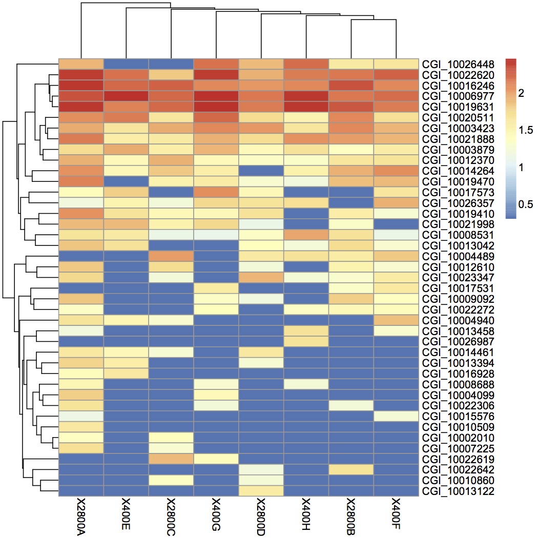
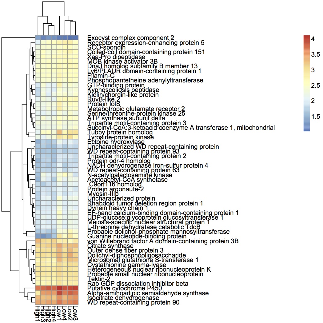
Heatmaps were made in R using pheatmap: clustering of samples (oysters) and variables (genes), average linkage clustering, euclidean distance, expression data are log+1 transformed. Not all the proteins from the proteomics data (this is just the subset with sig loadings in the NMDS) were represented in the RNA-seq data. Clustering did not follow treatment for any of the comparisons - only pCO2 is shown because that is really the only relevant one since no mechanically stressed oysters were sequenced using RNA-seq (although I looked at the expression of those genes as well). Expression levels at the transcriptomic level are different from expression levels at the proteomic level.
June 4, 2013
Secondary Stress: Buoyant weight
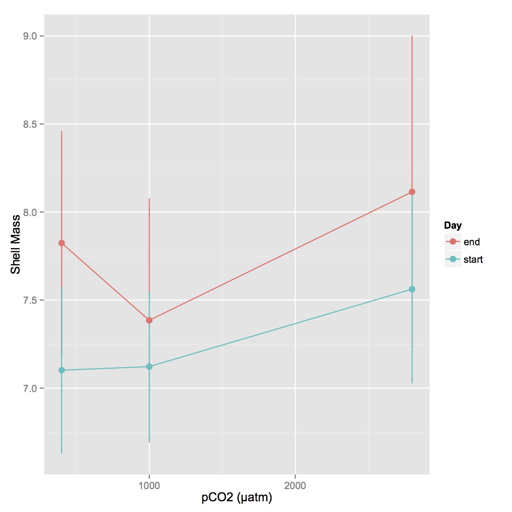
Created a new file that contains just data for BW for oysters at the beginning of the experiment and the end (29 days later). File name = oyster measurements BW.csv. Used this file to plot BW at the beginning and end of the experiment with 95% confidence intervals. Instructions and code for how to do this are from Cookbook for R (http://www.cookbook-r.com/Graphs/Plotting_means_and_error_bars_(ggplot2)/#Helper functions).
For the heat maps made 5/28, I annotated the groups of proteins. The pheatmap in R clusters proteins by similar expression profiles. I was trying to see if there were certain biological processes represented within those clusters. I looked at all the GO terms associated with proteins in each cluster and annotated those clusters with the most dominant processes found across multiple proteins.
May 28, 2013
Secondary Stress: Proteomics and buoyant weight
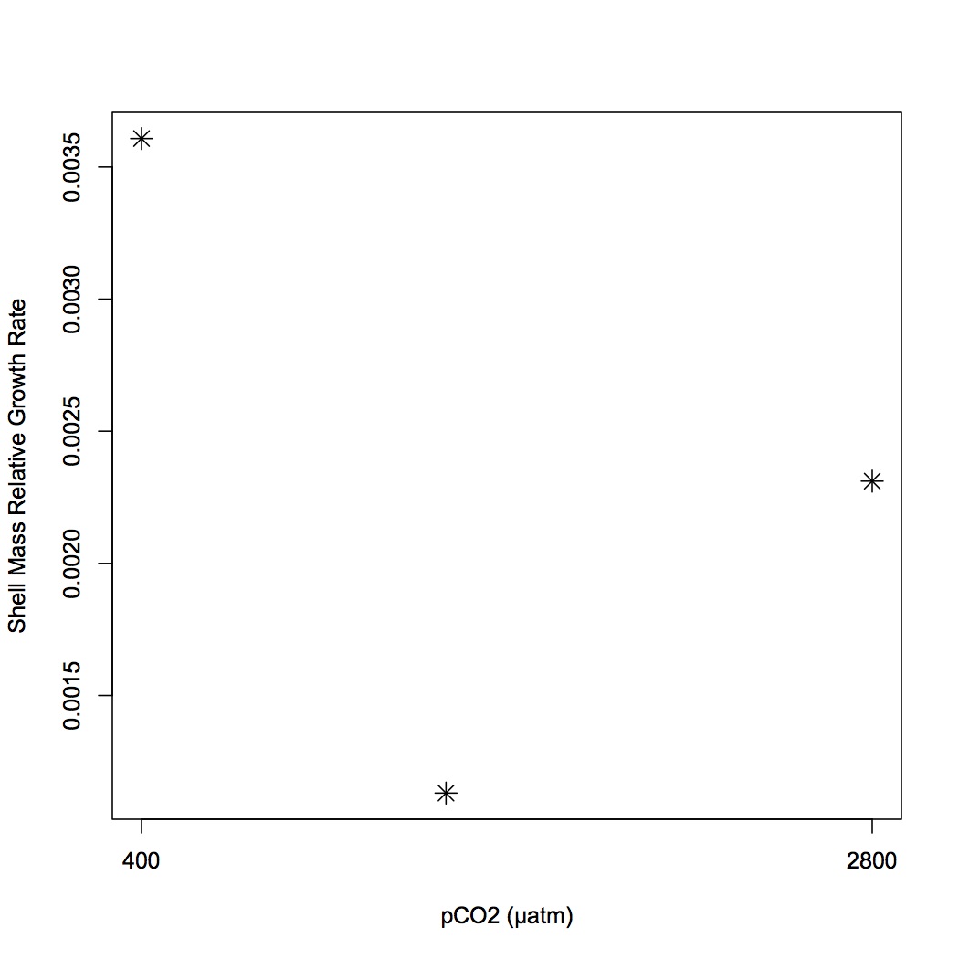
Did the same calculations for BW as I did previously for oyster length and width (see May 10, 2013). BW relative growth rate is greatest for oysters held at 400 µatm and least for oysters from 1000 µatm. 95% confidence intervals were also calculated using the following command in R: qnorm(0.975)*[stand dev of data]/sqrt(sample size). 95% were similar across time points for all 3 treatments.
Made heat maps of protein expression for proteins that are responsible for treatment response (see May 14, 2013) using pheatmap in R. Rows and columns are clustered using Euclidean distance and the average clustering method. Skyline expression data was log-transformed before use in the heat map. Below is an example from the pCO2 response data.
May 23, 2013
SQL Share
The following workflow shows how to use SQL share to analyze peptide expression data from Skyline.
1. JOIN DATA FILES INTO ONE FILE - FILES ARE JOINED ON TOP OF EACH OTHER. QUERY BELOW ADDS ANOTHER COLUMN WITH A FILE ID CORRESPONDING TO ORIGINATION FILE.
input files = prot data sample 1, prot data sample 2
output file = prot data all
SELECT
1 AS fileID, *
FROM [emmats@washington.edu].[prot data sample 1.txt]
UNION ALL
SELECT
2 AS fileID, *
FROM [emmats@washington.edu].[prot data sample 2.txt]
2. CREATE FILE OF UNIQUE PROTEIN PEPTIDE ASSOCIATIONS - this removes any redundant entries in the file
input file = prot data all (see step 1)
output file = TEST prot pep IDs
SELECT DISTINCT protein, [peptide sequence]
FROM [emmats@washington.edu].[prot data all]
3. FROM FILE OF ALL PROTEIN PEPTIDE ASSOCIATIONS, SUBSET ONLY THOSE THAT CORRESPOND TO PEPTIDES THAT HAVE A SINGLE PROTEIN MATCH - this maintains only informative peptides in the dataset
input file = TEST prot pep IDs (see step 2)
output file = protpeps
SELECT * FROM [TEST prot pep IDs] WHERE [peptide sequence] IN
(SELECT [peptide sequence]
FROM [emmats@washington.edu].[TEST prot pep IDs]
GROUP BY [peptide sequence]
HAVING COUNT (*) < 2)
4. JOINS DATA FILE (SPEC COUNTS) TO FILE WITH ONLY PEPTIDES MATCHING TO A SINGLE PROTEIN
input files = prot data all (step 1), protpeps (step 3)
output file = joined prot data
SELECT protein,[peptide sequence],
SUM (CASE WHEN fileID=1 then [tot indep spectra] else 0 end)
AS data1,
SUM (CASE WHEN fileID=2 then [tot indep spectra] else 0 end)
AS data2
FROM (
SELECT [prot data all].* FROM [emmats@washington.edu].[protpeps]
LEFT JOIN [prot data all]
ON [protpeps].[peptide sequence]=[prot data all].[peptide sequence])X
GROUP BY protein,[peptide sequence]
5. FINDS PROTEIN ABUNDANCE BASED ON SPEC COUNTS BY SUMMING ACROSS DATA COLUMNS
input file = joined prot data (step 4)
output file = sum spec counts
SELECT protein, [peptide sequence], data1+data2 AS sumallspec
FROM [emmats@washington.edu].[joined prot data]
6. ORDERS PROTEINS BY SPEC COUNTS (DESCENDING) AND THEN KEEPS ONLY FIRST 3 PEPTIDES (MOST ABUNDANT) FOR EACH PROTEIN
input file = sum spec counts (step 5)
output file = top 3 abundant peptides
SELECT * FROM
(SELECT *, ROW_NUMBER ()
OVER (PARTITION BY protein ORDER BY sumallspec DESC) AS pepabundance
FROM [emmats@washington.edu].[sum spec counts])x
WHERE pepabundance <= 3
To do next but not included in this workflow:
7. Join file top 3 abundant peptides (step 6) to file joined prot data (step 4) to create file of protein IDs, peptides, and data for individual oysters
8. Average peptide expression values for each protein so expression is on a per-protein basis (average across rows)
9. Average peptide expression values across technical replicates (average across columns)
May 15, 2013
Secondary Stress: Proteomics
Did separate anosims for the highly significant proteins within their specific comparisons (see 5/14/13): low vs. low X MS, high vs. high X MS, low vs. high. The 57 proteins are differentially expressed between low and high pCO2 (p=0.027) and the 22 proteins are differentially expressed in response to MS at low pCO2 (p=0.03), but expression is not different for the 28 proteins in response to MS at high pCO2.
Joined the list of highly significant eigenvector proteins with kegg pathway IDs in SQL.
SELECT * FROM [emmats@washington.edu].[highly significant proteins for anosim.csv]
LEFT JOIN [table_Cgigas_proteomev9_kegg_match]
ON [highly significant proteins for anosim.csv].Protein=[table_Cgigas_proteomev9_kegg_match].Column1
Loaded each list of KEGG IDs (for the 3 separate treatment comparisons) into iPath2 and saved as png files.
May 14, 2013
Secondary Stress: Proteomics
Joined files in SQL share to annotate Skyline daily data with kegg annotations:
SELECT * FROM [emmats@washington.edu].[Skyline daily with SPID]
LEFT JOIN [table_Cgigas_proteomev9_kegg_match]
ON [Skyline daily with SPID].protein=[table_Cgigas_proteomev9_kegg_match].[Column1]
Peptide peak areas were averaged across technical replicates and then across biological replicates so that each treatment has an expression value associated with each KEGG term. There are 2365 unique KEGG terms represented by this dataset (kegg with skyline daily expressions.txt).
Met with Julian to talk about how to determine which proteins (eigenvectors) are responsible for separation between treatment groups along a specific axis in NMDS. In the vector output (loadings), MDS1 and MDS2 refer to loadings on specific axes (1 and 2, respectively). Narrow down important proteins by p-value (choose <0.05 p-value for the number of variables that I have) and choose vectors with the highest (abs. value) loadings on the axis of interest. These will be the tails of the distribution of loadings - the extreme "outlier" values. These are the most important variables. Can choose them based on % of total or based on overall number of proteins of interest. For displaying, can create just those vectors on the plot or can list the important variables at the axis corners. Do ANOSIM on these most important variables. Also compare with PCoA (bray-curtis, log-transformed) since this method has axes that are independent of each other and can easily be separated. Does PCoA show the same patterns as NMDS?
p-value cutoff for NMDS loadings (output of eigenvector loadings is in 3 peps per protein area avgd) = 0.0099
MDS2 cutoff > or = |0.90|
For high vs. low pCO2, 57 proteins are highly significant. For High pCO2 vs. high x MS 28 proteins are highly significant and for low pCO2 vs low x MS, 22 proteins are highlyt significant.
Joined this file of highly significant eigenvector loadings with SPIDs, descriptions, GO, and GO slim terms in SQL.
SELECT * FROM [emmats@washington.edu].[highly significant NMDS loadings.txt]
LEFT JOIN [table_Cg proteome db evalue -10.txt]
ON [highly significant NMDS loadings.txt].Protein=[table_Cg proteome db evalue -10.txt].Protein
SELECT * FROM [emmats@washington.edu].[highly sig loadings with SPID]
LEFT JOIN [sr320@washington.edu].[qDOD Cgigas Gene Descriptions (Swiss-prot)]
ON [highly sig loadings with SPID].SPID=[qDOD Cgigas Gene Descriptions (Swiss-prot)].SPID
SELECT * FROM [emmats@washington.edu].[highly sig loadings with gene descriptions]
LEFT JOIN [dhalperi@washington.edu].[SPID_GOnumber.txt]
ON [highly sig loadings with gene descriptions].SPID=[dhalperi@washington.edu].[SPID_GOnumber.txt].A0A000
SELECT * FROM [emmats@washington.edu].[highly sig loadings with GO]
LEFT JOIN [sr320@washington.edu].[GO_to_GOslim]
ON [highly sig loadings with GO].[GO:0003824]=[sr320@washington.edu].[GO_to_GOslim].GO_id
May 10, 2013
Secondary Stress: oyster measurements
Yesterday I made files of oyster length, width, and adjusted buoyant weight from the sampling data from 2/11/12. The files only include oysters from treatments of pCO2 400, 1000, and 2800 µatm. For the time 0 data point, there is n=48 oysters for each treatment. for the time 1 month data point, there are n=48 for length and width (heat shocked oysters were included) but only 24 for buoyant weight because there is not forceps correction for the HS'd oysters in the data sheet.
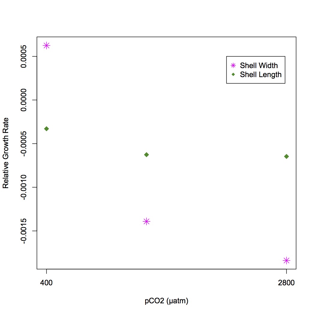
I am going to calculate the relative growth rate for length, width and buoyant weight from time =0 to 1 month later. This is based on the equation in Hoffmann & Poorter 2002 (http://aob.oxfordjournals.org/content/90/1/37.full.pdf), where they found that taking the ln of all the weights in a group and then taking the average was less biased than taking the ln of the average. Also calculated 95% CI for lengths and widths at time 0 and 1 month exposure for all 3 treatments (https://docs.google.com/spreadsheet/ccc?key=0An4PXFyBBnDEdHZTTm5QU2dtOFB6cWRndVdnajhJZGc&usp=sharing).
Secondary Stress: Epigenetics
The MeDip procedure is taken from this paper: Guerror-Basagna et al. http://www.plosone.org/article/info%3Adoi%2F10.1371%2Fjournal.pone.0013100
Jen designed primers for the medip PCR for caspase-3, catalase, cathepsin B, MAPK, and superoxide dismutase (SR IDs 1522-1531). All PCR products have at least one CpG in them. I created a database in Geneious of the oyster genome (v9_90) and searched all the primers (individually) against it. The top hit by far for each primer was the sequence it was designed for. When primers had a decent hit to another sequence, it was never the entire sequence of the primer that aligned and the other primer in the pair did not align to that same undesired sequence.
May 3, 2013
Secondary Stress: Epigenetics and Proteomics
Annotated the proteins associated with significant eigenvectors from the NMDS of low vs. high pCO2 (see 4/29) with SPID descriptions in SQL.
SELECT * FROM [emmats@washington.edu].[sig eigenvectors pCO2 SPID]
LEFT JOIN [table_TJGR_Gene_SPID_evalue_Description.txt]
ON [sig eigenvectors pCO2 SPID].CGID=[table_TJGR_Gene_SPID_evalue_Description.txt].[CGI Protein]
From this information, chose 49 proteins that looked interesting. Looked up their descriptions in Uniprot and narrowed down the list of interesting proteins to: catalase, heat shock protein 70 B2, peroxiredoxin-6, 60 kDa heat shock protein mitochondrial, v-type proton ATP-ase catalytic subunit A, caspase-3, heat shock protein beat-1, mitogen-activated protein kinase 7, superoxide dismutase [Cu-Zn] chloroplastic, cathepsin F, v-type proton ATP-ase subunit G, programmed cell death protein 5, cathepsin B. From these proteins we (Jen) are going to design primers for medip qPCR. The sequence amplified needs to contain at least one CpG so that if methylation is present it can be detected. Amplified fragments can be up to 700 bp long.
April 29, 2013
Secondary Stress: Proteomics
The file made 4/26 would not download completely. Contacted SQL support and they gave me a query that would work. Importantly, the avg command does not take the true average, but the average of the closest integers to the values in the data. The new query takes the true average.
SELECT protein
, avg(CAST([11_01 TotalArea] AS FLOAT))
, avg(CAST([11_02 TotalArea] AS FLOAT))
, avg(CAST([11_03 TotalArea] AS FLOAT))
, avg(CAST([2_01 TotalArea] AS FLOAT))
, avg(CAST([2_02 TotalArea] AS FLOAT))
, avg(CAST([2_03 TotalArea] AS FLOAT))
, avg(CAST([5_01 TotalArea] AS FLOAT))
, avg(CAST([5_02 TotalArea] AS FLOAT))
, avg(CAST([5_03 TotalArea] AS FLOAT))
, avg(CAST([8_01 TotalArea] AS FLOAT))
, avg(CAST([8_02 TotalArea] AS FLOAT))
, avg(CAST([8_03 TotalArea] AS FLOAT))
, avg(CAST([26_01 TotalArea] AS FLOAT))
, avg(CAST([26_02 TotalArea] AS FLOAT))
, avg(CAST([26_02 TotalArea] AS FLOAT))
, avg(CAST([26_03 TotalArea] AS FLOAT))
, avg(CAST([29_01 TotalArea] AS FLOAT))
, avg(CAST([29_02 TotalArea] AS FLOAT))
, avg(CAST([29_03 TotalArea] AS FLOAT))
, avg(CAST([32_01 TotalArea] AS FLOAT))
, avg(CAST([32_02 TotalArea] AS FLOAT))
, avg(CAST([32_03 TotalArea] AS FLOAT))
, avg(CAST([35_01 TotalArea] AS FLOAT))
, avg(CAST([35_02 TotalArea] AS FLOAT))
, avg(CAST([35_03 TotalArea] AS FLOAT))
, avg(CAST([221_01 TotalArea] AS FLOAT))
, avg(CAST([221_02 TotalArea] AS FLOAT))
, avg(CAST([221_03 TotalArea] AS FLOAT))
, avg(CAST([224_01 TotalArea] AS FLOAT))
, avg(CAST([224_02 TotalArea] AS FLOAT))
, avg(CAST([224_03 TotalArea] AS FLOAT))
, avg(CAST([227_01 TotalArea] AS FLOAT))
, avg(CAST([227_02 TotalArea] AS FLOAT))
, avg(CAST([227_03 TotalArea] AS FLOAT))
, avg(CAST([230_01 TotalArea] AS FLOAT))
, avg(CAST([230_02 TotalArea] AS FLOAT))
, avg(CAST([230_02 TotalArea] AS FLOAT))
, avg(CAST([242_01 TotalArea] AS FLOAT))
, avg(CAST([242_02 TotalArea] AS FLOAT))
, avg(CAST([242_03 TotalArea] AS FLOAT))
, avg(CAST([245_01 TotalArea] AS FLOAT))
, avg(CAST([245_02 TotalArea] AS FLOAT))
, avg(CAST([245_03 TotalArea] AS FLOAT))
, avg(CAST([248_01 TotalArea] AS FLOAT))
, avg(CAST([248_02 TotalArea] AS FLOAT))
, avg(CAST([248_03 TotalArea] AS FLOAT))
, avg(CAST([251_01 TotalArea] AS FLOAT))
, avg(CAST([251_02 TotalArea] AS FLOAT))
, avg(CAST([251_03 TotalArea] AS FLOAT))
FROM [che625@washington.edu].[3 peps per protein.txt]
GROUP BY protein
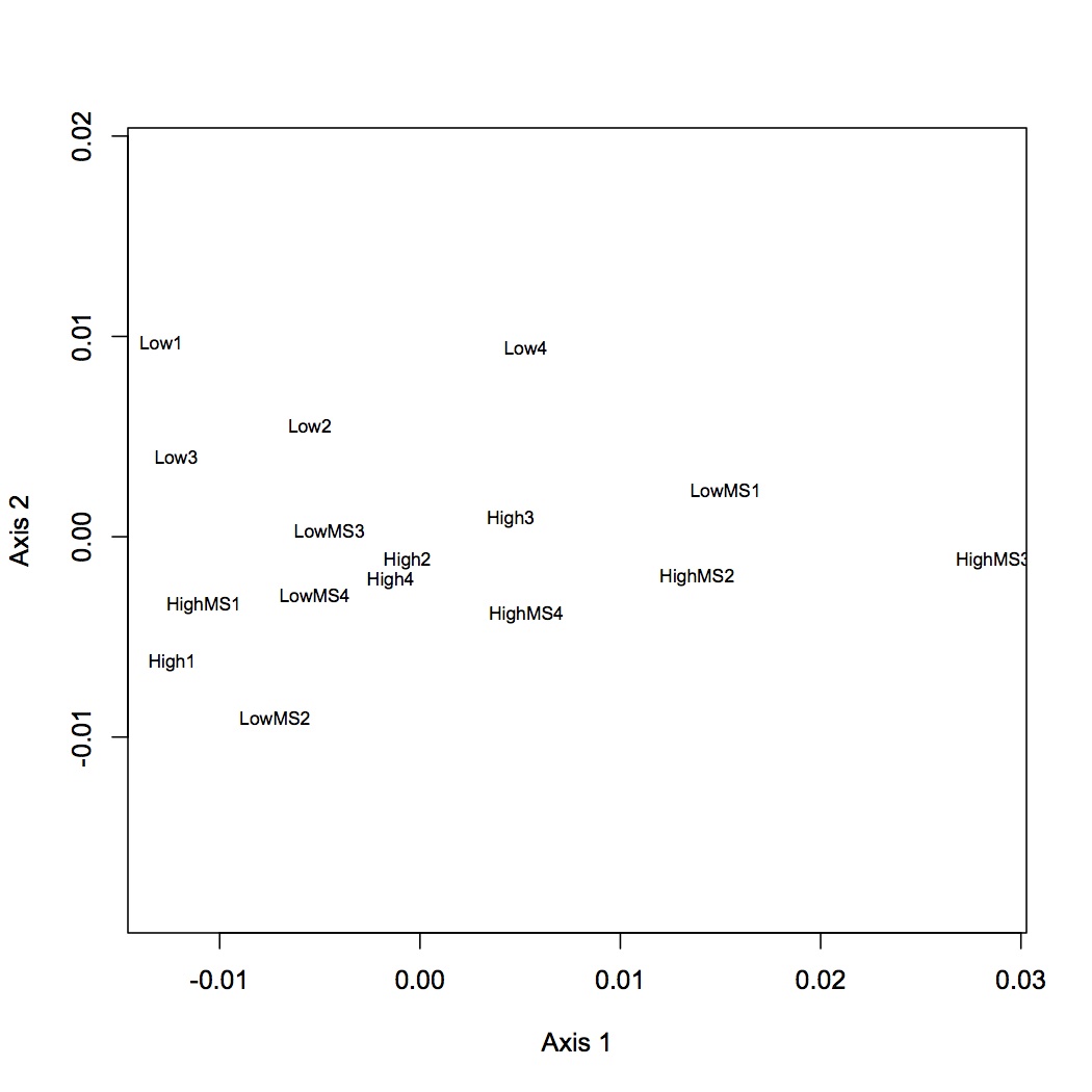
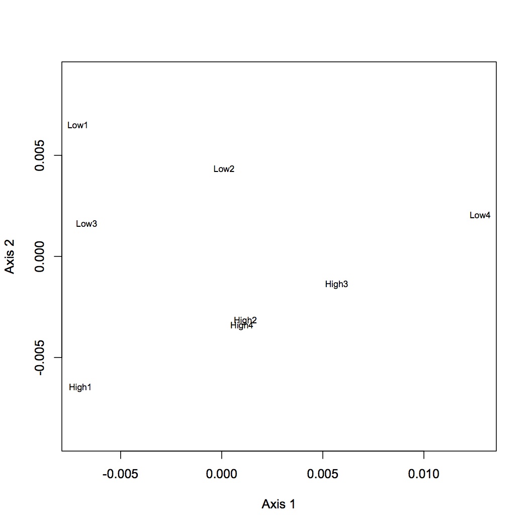
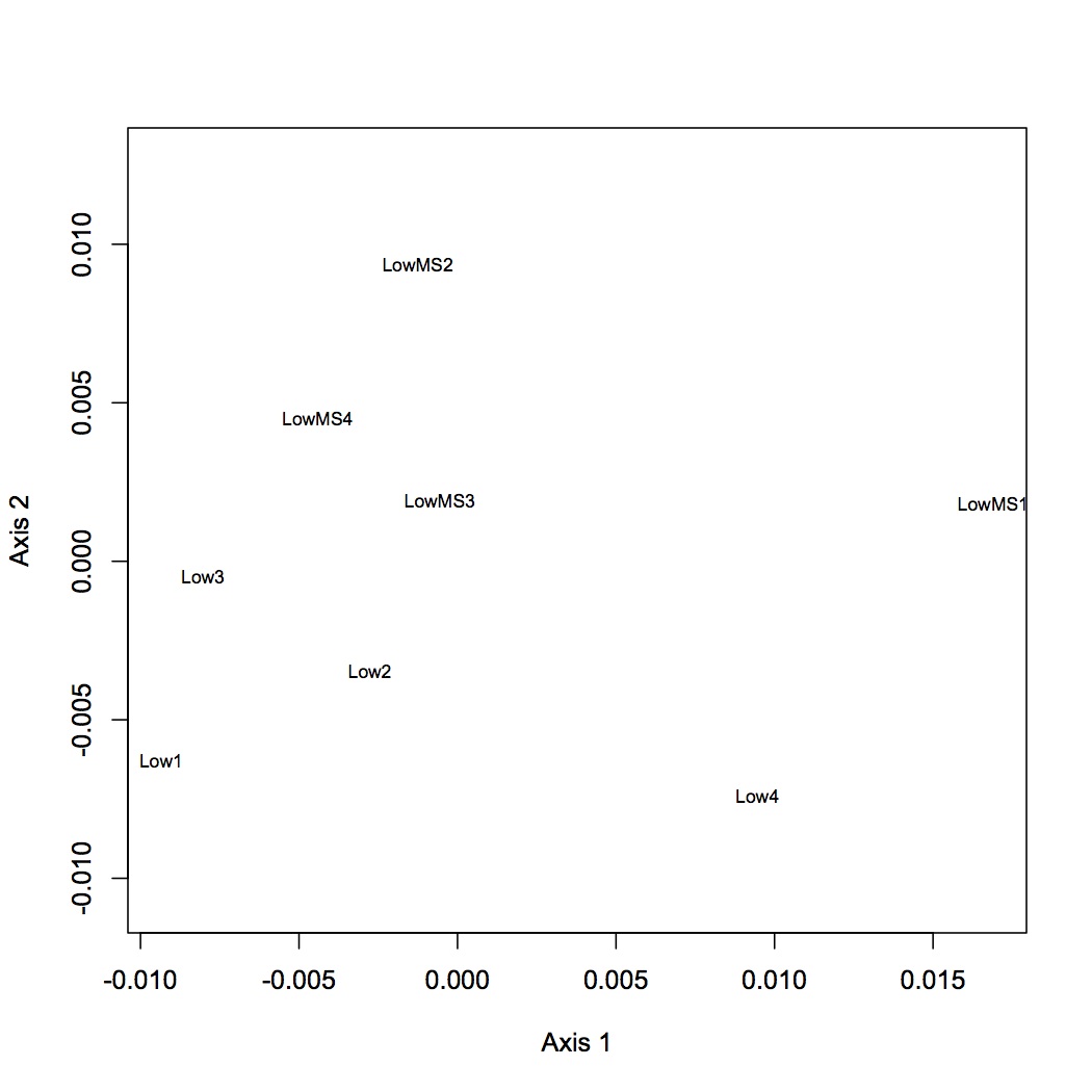
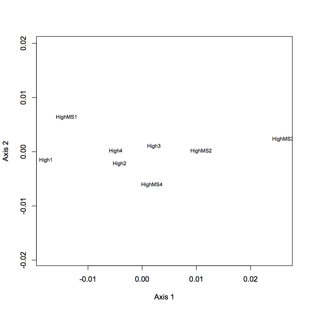
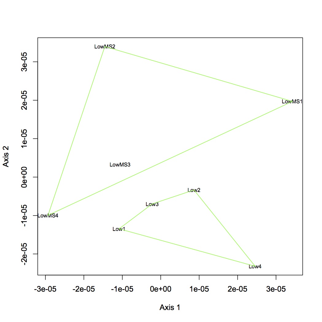
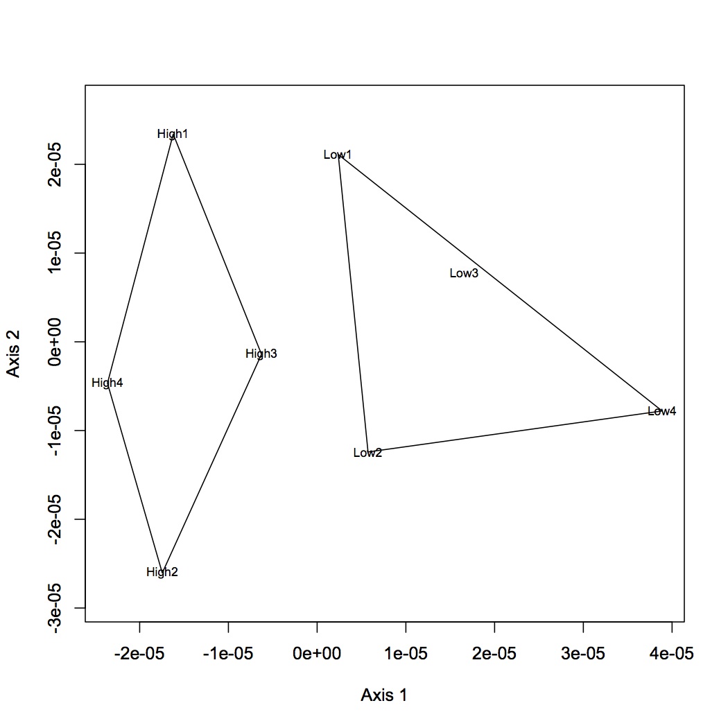
2677 proteins are in the Skyline dataset. Averaged Skyline peptide areas across technical replicates. Made NMDS plots of all treatments together, low vs. high pCO2, low pCO2 vs. low MS, and high pCO2 vs high MS. ANOSIM showed no significant differences among proteomic profiles for the different treatments (although low vs. high pCO2 was p=0.06). Also found eigenvector loadings for each plot to determine significance of the contribution of each protein in contributing to the division of the objects (oysters) in multivariate space.
All Treatments
Low vs. High pCO2
Low pCO2 vs. Low x MS
High pCO2 vs. High x MS
Annotated the gill proteome with SPID in SQL share. Also annotated with GO and GO Slim terms.
SELECT * FROM [emmats@washington.edu].[3 peps per protein area avgd]
LEFT JOIN [Cg proteome db evalue -10.txt]
ON [3 peps per protein area avgd].protein=[Cg proteome db evalue -10.txt].Protein
SELECT * FROM [emmats@washington.edu].[gill proteome with SPID.txt]
LEFT JOIN [dhalperi@washington.edu].[SPID_GOnumber.txt]
ON [gill proteome with SPID.txt].SPID=[dhalperi@washington.edu].[SPID_GOnumber.txt].A0A000
SELECT * FROM [emmats@washington.edu].[gill proteome with GO]
LEFT JOIN [sr320@washington.edu].[GO_to_GOslim]
ON [gill proteome with GO].[GO:0003824]=[sr320@washington.edu].[GO_to_GOslim].GO_id
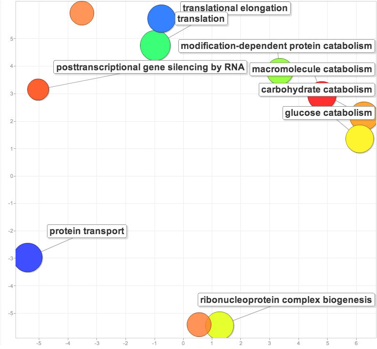
Using DAVID (GO BP_FAT) found biological processes that are enriched in the gill proteome vs. the entire proteome. The gene list (gill proteome) was the unique SPIDs used to annotate the 2,677 gill proteins and the background were the SPID annotations for the entire proteome (from Zhang et al.). Visualized in Revigo.
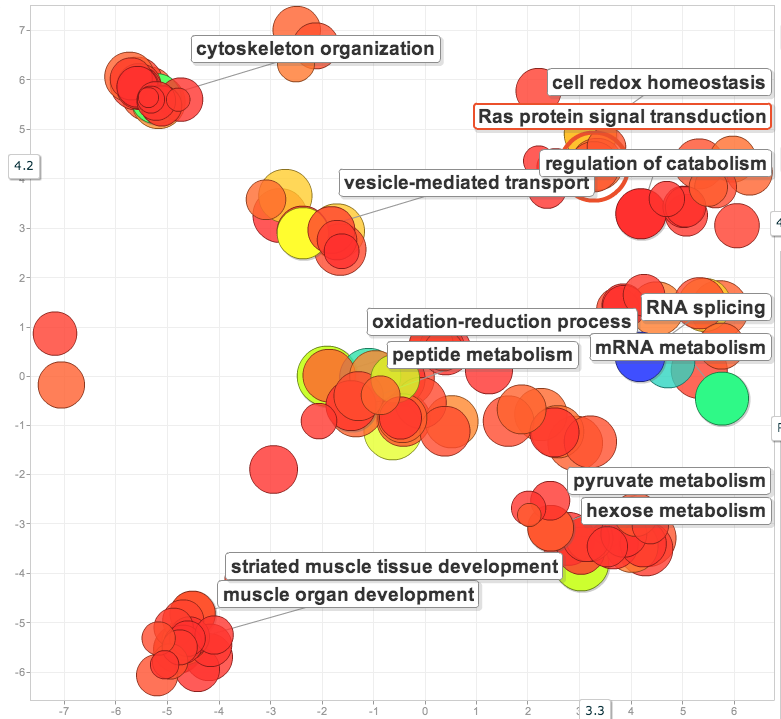
Based on the significant eigenvectors (p<0.05) for the low vs. high pCO2 NMDS, found enrichment versus the entire gill proteome.
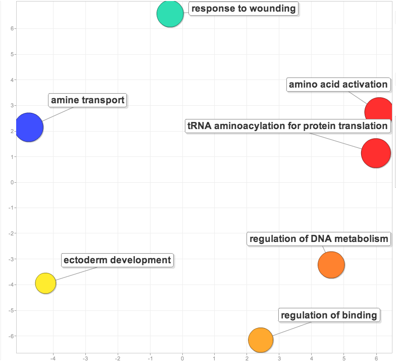
Compared the list of proteins corresponding to significant eigenvectors for low pCO2 vs. low x MS and high pCO2 vs. high X MS. For the proteins unique to the high X MS response (i.e. were not shared between the 2 lists), found the enrichment of biological processes compared to the entire gill proteome.
April 26, 2013
Secondary Stress: Proteomics
For the Skyline output, removed all peptides that matched to multiple proteins. Then kept only top 3 most abundant peptides per protein (abundance was determined based on total area across all replicates).
Averaged peptide peak areas by protein in SQL
SELECT protein, avg([11_01 TotalArea]), avg([11_02 TotalArea]), avg([11_03 TotalArea]), avg([2_01 TotalArea]), avg([2_02 TotalArea]), avg([2_03 TotalArea]), avg([5_01 TotalArea]), avg([5_02 TotalArea]), avg([5_03 TotalArea]), avg([8_01 TotalArea]), avg([8_02 TotalArea]), avg([8_03 TotalArea]), avg([26_01 TotalArea]), avg([26_02 TotalArea]), avg([26_02 TotalArea]), avg([26_03 TotalArea]), avg([29_01 TotalArea]), avg([29_02 TotalArea]), avg([29_03 TotalArea]), avg([32_01 TotalArea]), avg([32_02 TotalArea]), avg([32_03 TotalArea]), avg([35_01 TotalArea]), avg([35_02 TotalArea]), avg([35_03 TotalArea]), avg([221_01 TotalArea]), avg([221_02 TotalArea]), avg([221_03 TotalArea]), avg([224_01 TotalArea]), avg([224_02 TotalArea]), avg([224_03 TotalArea]), avg([227_01 TotalArea]), avg([227_02 TotalArea]), avg([227_03 TotalArea]), avg([230_01 TotalArea]), avg([230_02 TotalArea]), avg([230_02 TotalArea]), avg([242_01 TotalArea]), avg([242_02 TotalArea]), avg([242_03 TotalArea]), avg([245_01 TotalArea]), avg([245_02 TotalArea]), avg([245_03 TotalArea]), avg([248_01 TotalArea]), avg([248_02 TotalArea]), avg([248_03 TotalArea]), avg([251_01 TotalArea]), avg([251_02 TotalArea]), avg([251_03 TotalArea]) FROM [che625@washington.edu].[3 peps per protein.txt]
Group by protein
April 18, 2013
Secondary Stress: Proteomics
Created a list of non-redundant protein-peptide associations. This is a combination of all the peptide sequences and their associated proteins sequenced across all injections. The file is called ProtPep for all oysters.
Joined ProtPep file with file of all peak areas for sequenced peptides. This file has been edited so that peak areas are only for the precursor ion (not M+1 or M+2) and #N/A were replaced with 0. The joined file is peptide peak areas with associated proteins.
April 17, 2013
Secondary Stress: Proteomics
Created a report template called Oyster Report 1 that includes the information: Peptide sequence, precursor best retention time, precursor total area, protein name, precursor charge, percursor Mz, transition product charge, transition product Mz, transition fragmentation, checked box for pivot replicate name. Exported all samples and replicates using this template.
April 16, 2013
Secondary Stress: Proteomics
Brendan gave me access to Skyline daily, a beta version of Skyline that has a lot of improvements compared to the public release. He had fixed it so that it would take all my data files. I set up all the settings today (see below, also saved in a text file) and imported all the raw data files. The library is called Oyster_proteins_daily. All of the v9 "interact" files were used to construct the library (the C. gigas v9 proteome was used in Sequest and only proteins with a probability of at least 0.9 were included - check that actually 0.9). In the spectral library explorer, clicked "add all" to ad all the peptides to the protein/peptide tree (did not include peptides that do not match the current filters). Selected all the peptides in the tree then Edit > Refine to remove duplicate peptides and empty proteins.
Peptide Settings
Digestion: Enzyme = Trypsin [KR | P]
Max missed cleavages = 2
Background proteome = None
Modifications: Carbamidomethyl (C), Oxidation (M) - variable
Max variable mods = 3
Max neutral losses = 1
Isotop label type = heavy
Internal standard type = heavy
Library: Keep redundant library
Cut-off score = 0.95
Pick peptides matching Library
Transition Settings
Predition: Precursor mass = Monoisotopic
Product ion mass = Monoisotopic
Collision energy = Thermo TSQ Vantage
Declustering potential = None
Filter: Precursor charges = 2,3,4
Ion charges = 1,2,3
Ion types = p
Product ions: From m/z/ > precursor
To 3 ions
Always add N-terminal to Proline
Auto-select all matching transitions
Library: Ion match tolerance = 0.5 Th
Do not check "If a library spectrum is available, pick its most intense ions"
Instrument: Min m/z = 50 Th, Max m/z = 2000 Th
Method match tolerance m/z = 0.055 Th
Full-Scan: Isotope peaks included = Count
Precursor mass analyzer = Orbitrap
Peaks = 3
Resolving power = 60,000 at 400 Th
Isotope labeling enrichment = Default
Acquisition method = None
Use only scans within 5 minutes of MS/MS IDs
April 13, 2013
Secondary Stress: Proteomics
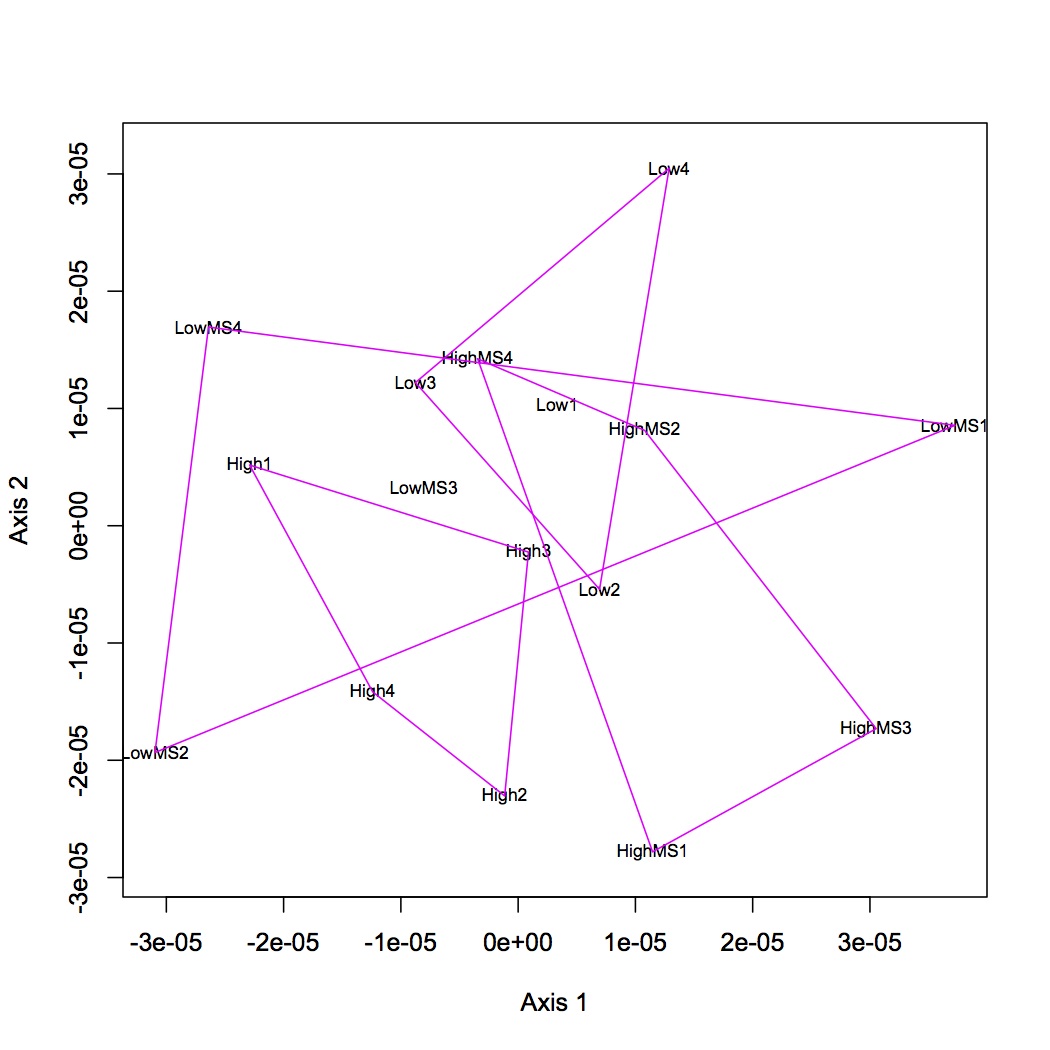
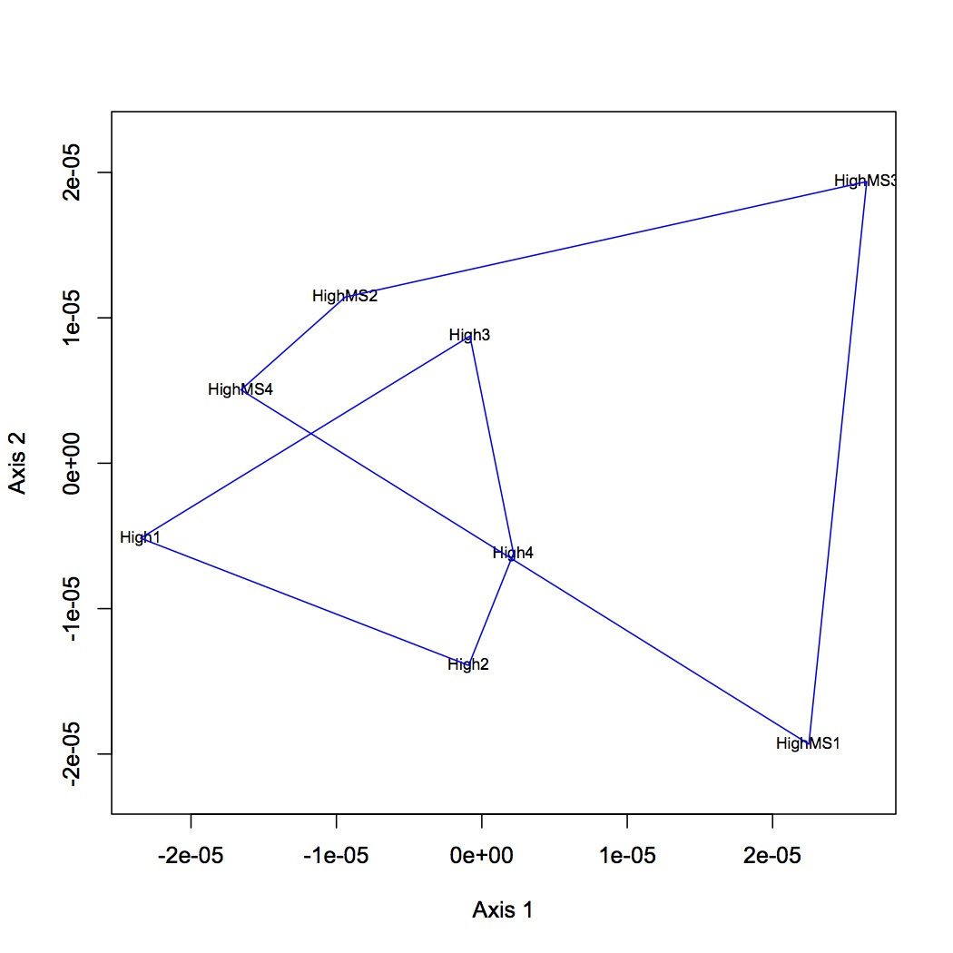
Proteins were analyzed only if they had at least 2 unique peptide hits in a technical replicate and if they had at least 8 spectral counts across all replicates. Calculated NSAF for all proteins and analyzed using NMDS. Made NMDS (kept all proteins for analysis) of all 4 treatments, MS at high and low pCO2, and just comparison of pCO2. (R file is called NSAF proteomics.) ANOSIM was done for all 4 treatments, low pCO2 vs. MS, high pCO2 vs. MS, and high vs. low pCO2.
April 12, 2013
Secondary Stress: Epigenetics
Yesterday samples were nanodropped 1 time and these concentrations were used to calculate how much DNA to shear. The samples should be between 8-20 µg and be 100 µl. 103B230 has the lowest concentration of 126.64 ng/µl and 100 µl of this sample contains 12.7 µg of DNA. 101B2 and 101B5 are the supernatant after the extracted and partially solubilized samples were spun down (see 4/11/13).
| Sample |
ng/µl |
µg/µl |
vol. for 12.7 µg |
vol H2O for 100 µl |
| 101B2 |
382.56 |
0.383 |
33.2 |
66.8 |
| 101B5 |
306.39 |
0.306 |
44.5 |
58.5 |
| 101B8 |
322.15 |
0.322 |
39.4 |
60.6 |
| 103B224 |
330.52 |
0.331 |
33.4 |
61.6 |
| 103B227 |
294.41 |
0.294 |
46.6 |
53.4 |
| 103B230 |
126.64 |
0.127 |
100 |
0 |
Secondary Stress: Proteomics
For file created 4/10/13, removed proteins within a technical replicate that had fewer than 2 unique peptide hits. Also removed proteins that had fewer than 8 total spectral counts across all injections (48). This leaves 1459 proteins. Found total SpC for each oyster by taking sum across technical replicates. Joined this file with protein lengths in SQL share.
SELECT * FROM [emmats@washington.edu].[all oysters SpC.txt]
LEFT JOIN [protein length.txt]
ON [all oysters SpC.txt].Protein=[protein length.txt].protein
April 11, 2013
Secondary Stress: Epigenetics
Continued with DNA extraction as described 2/8/13. Samples were solubilized in 200 µl water at 55C for 10 minutes. 101B2 and 101B5 were still a little viscous with some visible chunks in them after this. They also had the highest concentrations on the nanodrop (>500 and >400 ng/µl). I added 100 µl of water to each and spun them at 5,000xg for 5 minutes and removed the supernatant to a new tube, also keeping the "pellet". The supernatant caused the same error on the nanodrop that the entire mixture did. All samples are stored at -20C in Emma's -20 box started 5/10/11.
April 10, 2013
Secondary Stress: Proteomics
Joined together all tables of unique spectral counts and total spectral counts for each replicate (n=48) to a backbone of a unique list of proteins identified in SQLshare. File is called All SpC joined for 16 oysters.
SELECT *
FROM [emmats@washington.edu].[all sequenced proteins all treatments.txt]
LEFT JOIN [table_101B_2_01.txt]
ON [all sequenced proteins all treatments.txt].[All Proteins]=[table_101B_2_01.txt].protein
LEFT JOIN [table_101B_2_02.txt]
ON [all sequenced proteins all treatments.txt].[All Proteins]=[table_101B_2_02.txt].protein
LEFT JOIN [table_101B_2_03.txt]
ON [all sequenced proteins all treatments.txt].[All Proteins]=[table_101B_2_03.txt].protein
LEFT JOIN [table_101B_5_01.txt]
ON [all sequenced proteins all treatments.txt].[All Proteins]=[table_101B_5_01.txt].protein
LEFT JOIN [table_101B_5_02.txt]
ON [all sequenced proteins all treatments.txt].[All Proteins]=[table_101B_5_02.txt].protein
LEFT JOIN [table_101B_5_03.txt]
ON [all sequenced proteins all treatments.txt].[All Proteins]=[table_101B_5_03.txt].protein
LEFT JOIN [table_101B_8_01.txt]
ON [all sequenced proteins all treatments.txt].[All Proteins]=[table_101B_8_01.txt].protein
LEFT JOIN [table_101B_8_02.txt]
ON [all sequenced proteins all treatments.txt].[All Proteins]=[table_101B_8_02.txt].protein
LEFT JOIN [table_101B_8_03.txt]
ON [all sequenced proteins all treatments.txt].[All Proteins]=[table_101B_8_03.txt].protein
LEFT JOIN [table_101B_11_01.txt]
ON [all sequenced proteins all treatments.txt].[All Proteins]=[table_101B_11_01.txt].protein
LEFT JOIN [table_101B_11_02.txt]
ON [all sequenced proteins all treatments.txt].[All Proteins]=[table_101B_11_02.txt].protein
LEFT JOIN [table_101B_11_03.txt]
ON [all sequenced proteins all treatments.txt].[All Proteins]=[table_101B_11_03.txt].protein
LEFT JOIN [table_101B_26_01.txt]
ON [all sequenced proteins all treatments.txt].[All Proteins]=[table_101B_26_01.txt].protein
LEFT JOIN [table_101B_26_02.txt]
ON [all sequenced proteins all treatments.txt].[All Proteins]=[table_101B_26_02.txt].protein
LEFT JOIN [table_101B_26_03.txt]
ON [all sequenced proteins all treatments.txt].[All Proteins]=[table_101B_26_03.txt].protein
LEFT JOIN [table_101B_29_01.txt]
ON [all sequenced proteins all treatments.txt].[All Proteins]=[table_101B_29_01.txt].protein
LEFT JOIN [table_101B_29_02.txt]
ON [all sequenced proteins all treatments.txt].[All Proteins]=[table_101B_29_02.txt].protein
LEFT JOIN [table_101B_29_03.txt]
ON [all sequenced proteins all treatments.txt].[All Proteins]=[table_101B_29_03.txt].protein
LEFT JOIN [table_101B_32_01.txt]
ON [all sequenced proteins all treatments.txt].[All Proteins]=[table_101B_32_01.txt].protein
LEFT JOIN [table_101B_32_02.txt]
ON [all sequenced proteins all treatments.txt].[All Proteins]=[table_101B_32_02.txt].protein
LEFT JOIN [table_101B_32_03.txt]
ON [all sequenced proteins all treatments.txt].[All Proteins]=[table_101B_32_03.txt].protein
LEFT JOIN [table_101B_35_01.txt]
ON [all sequenced proteins all treatments.txt].[All Proteins]=[table_101B_35_01.txt].protein
LEFT JOIN [table_101B_35_02.txt]
ON [all sequenced proteins all treatments.txt].[All Proteins]=[table_101B_35_02.txt].protein
LEFT JOIN [table_101B_35_03.txt]
ON [all sequenced proteins all treatments.txt].[All Proteins]=[table_101B_35_03.txt].protein
LEFT JOIN [table_103B_221_01.txt]
ON [all sequenced proteins all treatments.txt].[All Proteins]=[table_103B_221_01.txt].protein
LEFT JOIN [table_103B_221_02.txt]
ON [all sequenced proteins all treatments.txt].[All Proteins]=[table_103B_221_02.txt].protein
LEFT JOIN [table_103B_221_03.txt]
ON [all sequenced proteins all treatments.txt].[All Proteins]=[table_103B_221_03.txt].protein
LEFT JOIN [table_103B_224_01.txt]
ON [all sequenced proteins all treatments.txt].[All Proteins]=[table_103B_224_01.txt].protein
LEFT JOIN [table_103B_224_02.txt]
ON [all sequenced proteins all treatments.txt].[All Proteins]=[table_103B_224_02.txt].protein
LEFT JOIN [table_103B_224_03.txt]
ON [all sequenced proteins all treatments.txt].[All Proteins]=[table_103B_224_03.txt].protein
LEFT JOIN [table_103B_227_01.txt]
ON [all sequenced proteins all treatments.txt].[All Proteins]=[table_103B_227_01.txt].protein
LEFT JOIN [table_103B_227_02.txt]
ON [all sequenced proteins all treatments.txt].[All Proteins]=[table_103B_227_02.txt].protein
LEFT JOIN [table_103B_227_03.txt]
ON [all sequenced proteins all treatments.txt].[All Proteins]=[table_103B_227_03.txt].protein
LEFT JOIN [table_103B_230_01.txt]
ON [all sequenced proteins all treatments.txt].[All Proteins]=[table_103B_230_01.txt].protein
LEFT JOIN [table_103B_230_02.txt]
ON [all sequenced proteins all treatments.txt].[All Proteins]=[table_103B_230_02.txt].protein
LEFT JOIN [table_103B_230_03.txt]
ON [all sequenced proteins all treatments.txt].[All Proteins]=[table_103B_230_03.txt].protein
LEFT JOIN [table_103B_242_01.txt]
ON [all sequenced proteins all treatments.txt].[All Proteins]=[table_103B_242_01.txt].protein
LEFT JOIN [table_103B_242_02.txt]
ON [all sequenced proteins all treatments.txt].[All Proteins]=[table_103B_242_02.txt].protein
LEFT JOIN [table_103B_242_03.txt]
ON [all sequenced proteins all treatments.txt].[All Proteins]=[table_103B_242_03.txt].protein
LEFT JOIN [table_103B_245_01.txt]
ON [all sequenced proteins all treatments.txt].[All Proteins]=[table_103B_245_01.txt].protein
LEFT JOIN [table_103B_245_02.txt]
ON [all sequenced proteins all treatments.txt].[All Proteins]=[table_103B_245_02.txt].protein
LEFT JOIN [table_103B_245_03.txt]
ON [all sequenced proteins all treatments.txt].[All Proteins]=[table_103B_245_03.txt].protein
LEFT JOIN [table_103B_248_01.txt]
ON [all sequenced proteins all treatments.txt].[All Proteins]=[table_103B_248_01.txt].protein
LEFT JOIN [table_103B_248_02.txt]
ON [all sequenced proteins all treatments.txt].[All Proteins]=[table_103B_248_02.txt].protein
LEFT JOIN [table_103B_248_03.txt]
ON [all sequenced proteins all treatments.txt].[All Proteins]=[table_103B_248_03.txt].protein
LEFT JOIN [table_103B_251_01.txt]
ON [all sequenced proteins all treatments.txt].[All Proteins]=[table_103B_251_01.txt].protein
LEFT JOIN [table_103B_251_02.txt]
ON [all sequenced proteins all treatments.txt].[All Proteins]=[table_103B_251_02.txt].protein
LEFT JOIN [table_103B_251_03.txt]
ON [all sequenced proteins all treatments.txt].[All Proteins]=[table_103B_251_03.txt].protein
Secondary Stress: Epigenetics
Extracted DNA from 6 oysters to do medip. These 6 oysters are part of the 16 that were used for proteomics in August 2012. Posterior gill tissue was used from high pCO2 sample numbers 101B2, 101B5, 101B8 and low pCO2 number 103B224, 103B227, and 103B230. Gill tissue was homogenized in 0.5 mL of DNazol using a sterile pestle. 0.5 mL more DNazol and 2.35 µl proteinase K were added and tubes were inverted to mix. Tubes were incubated on the rotating thingy overnight at room temperature.