GBS help

I. Bioinformatic analysis

The original image data of sequencing was converted to sequences in fastq format by base calling. Every read in fastq file was described by four lines as following:

@FCB068CABXX:6:1101:1403:2159#TAGGTTAT/1
GTAGAAGACTTATAGATTAAAATTCTCCAACATATAGATGTCCTTACACCGTTTTCCTTTGCTCAGCAGGCTCCGTGTTTGCTTGTCCTT
+
c`bcc_c^ccde_df\c_aeff`ffcfffdfedadca^`b_eed`fe\fed\babdba^Yeebeccfdeae_eec^dbXbda`]bcbebc

Line 1 and 3 are names of reads generated by the sequence analyzer(The name after "+" was deleted in order to save storage); Line 2 is sequences; Line 4 is quality values of bases, which equals to ASCII code in line 4 minus 64. For example, the ASCII code of "c" is 99, then its base quality value is 35. The correlation between sequencing error rate and quality values of bases generated by Illumina HiSeq™ 2000 was shown in Table 1. If the sequencing error rate is E and Illunima HiSeq™ 2000 base quality value is sQ, the equation will be as following:

1)Remove reads with adaptors;
2)Remove low quality reads (i.e. reads with more than 50% bases whose quality value are less than or equal to 5);
3)Classify reads with barcode sequences which verifies between samples;
4)Remove the reads that cannot be identified with barcode sequnces.

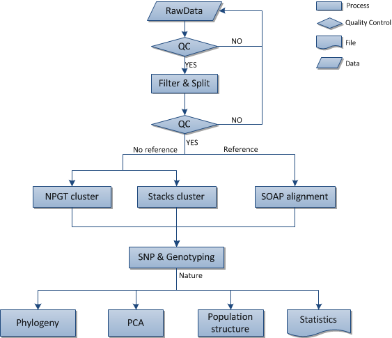
For species with reference genome sequences, clean reads will be mapped against the reference genome sequences with SOAPaligner^[1](http://soap.genomics.org.cn).The average depth and coverage will be calculated according to the mapping result. For reads which cannot be mapped, following steps will be taken until the processed reads have alignment on reference sequences: Firstly, remove the first one base and last two bases of read and map it against reference sequences, if the processed reads still can't match on sequences, the last two bases will be removed repeatedly until the alignment is found. The processed reads shorter than 40bp will be removed if there is still no alignment.

For species without reference genome sequences, we will use self-developed NPGT packages or Stacks^[2](http://creskolab.uoregon.edu/stacks/)to cluster reads1,and do the next SNP detection According to the cluster results.

For species with reference genome sequences, Considering data characteristics, quality of sequencing and influence of experiments, soapsnp^[3]will be used for SNP detection, during which a Bayesian model is utilized and every possible genotype probabilities will be calculated based on the observed data. Genotype with the maximum probability will be selected as final genotype and a quality value will be provided to measure the accuracy. Consensus sequences(Sequences with alignment information on each base) will be generated based on genotypes.Polymorphic loci on reference sequences will be filtered based on consensus sequences. The loci meeting the following criteria will be retained:

1)Quality value had to be greater than or equal to 20.
2)Approximate copy number of flanking sequences had to be less than or equal to 1.5.
3)SNPs had to be at least 5bp away from each other.
4)Rank sum test statistic had to be greater than or equal to 0.05.

For species with no reference genome sequences, we use radsnp (a package in NPGT) on reads1 for SNP detection.

We integrate SNP results of all samples ,filter out the SNP with missing rate greater than 50% and generate genotying list.

Phylogenetic tree (also known as evolutionary tree) is cladogram or tree which describes the evolutionary relationship among groups. The SNPs can be used to calculate the distance between the populations after SNP detection. P (the distance) between the two individuals i and j is calculated by the following formula:

L is the length of SNPs area. Hypothetically the allele is A/C in position 1, then:

We use MEGA5.0^[4](http://mega.software.informer.com/5.0/)or TreeBeST(http://treesoft.sourceforge.net/treebest.shtml)or PHYLIP(http://evolution.genetics.washington.edu/phylip.html) software to calculate the distance matrix, based on which we build phylogeny tree using joining method. The bootstrap values is set to 1000.

Principal Component Analysis (PCA) is a mathematical procedure that uses orthogonal transformation to convert a set of observations of possibly correlated variables into a set of values of linearly uncorrelated variables called principal components. We use PCA on autosomal SNP data only and ignore loci with more than two allels or mismatch to reduce interference.

In individual i,d_ikrepresents the information about SNP on the site k.If the individual i and reference alleles are homozygous,d_ik=0;If it is a heterozygote,d_ik=1;If the individual with the non reference allele is homozygous,d_ik=2.M is a n * S matrix that include standard genotype:

E(d_ik)is the average value of d_k,the individual sample's n×n matrix covariance is calculated in formula: X=MM^T/S. X's eigenvector decomposition is completed by R's functions.We use EIGENSOFT^[5](http://genetics.med.harvard.edu/reich/Reich_Lab/Software.html) built-in package twstats to perform Tracey - Widom test and get the result of the eigenvector significance analysis.

Population genetic structure refers to a kind of non-random distribution of genetic variation in the species or groups. According to the geographical distribution, or other standards, a group can be divided into several subgroups.Population structure analysis can helps to explain the evolutionary process and found which subgroup the individual belongs to based on the genotype and phenotype correlation research.FRAPPE^[6]use the maximum likelihood method to interfer each individual's genetic ancestry assuming that the individuals come from the group of the K ancestors.

II. Refrence

1. Li R.,Yu C.,Li Y.,et al.(2009).SOAP2:An improved ultrafast tool for short read alignment.Bioinformatics,25(15).1966-1967.
2. J. Catchen,A. Amores,P. Hohenlohe,W. Cresko, and J. Postlethwait.Stacks:building and genotyping loci denovo from short-read sequences.G3: Genes,Genomes,Genetics,1:171-182,2011.
3. Ruiqiang Li, Yingrui Li, Xiaodong Fang,et al.(2009)SNP detection for massively parallel whole-genome resequencing Genome Res.,doi:10.1101/gr.088013.108.
4. Koich iro Tamura,et al. MEGA4:Molecular Evolutionary Genetics Analysis (MEGA) Software Version 4.0.Mol Biol Evol (2007)24(8):1596-1599.doi:10.1093/molbev/msm092.
5. Alkes L Price, Patterson NJ,Plenge RM,Weinblatt ME,Shadick NA,Reich D.(2006) Principal components analysis corrects for stratification in genome-wide association studies.Nature Genetics 38,904-909.
6. Tang,H.,Peng,J.,Wang,P.& Risch,N.J. Estimation of individual admixture:analytical and study design considerations.Genet.Epidemiol.28,289-301(2005).

III. The list of analysis result

upload
|---- Cleandata                     clean reads directory
|     |---  A.fq.gz                 sample A clean data
|     |---  B.fq.gz                 sample B clean data
|---- Data.stat.xls                 all the samples data statistics list
|---- SNP.stat.xls                  all the samples SNP statistics list
|---- Genotype.xls                  all the samples genotyping statistics list
|---- tree                          Phylogenetic tree result directory
|     |---  nj_tree.out.tre.png     Phylogenetic tree analysis result (png format)
|     |---  nj_tree.out.tre.svg     Phylogenetic tree analysis result(SVG format)
|---- PCA                           PCA result directory
|     |---  1-2.png                 the contribution rate of component 1 and 2
|     |---  1-3.png                 the contribution rate of component 1 and 3
|     |---  m-n.png                 the contribution rate of component m and n
|---- structure                     Population structure result directory
|     |---  STRUCTURE.png           Population structureanalysis result (png format)
|     |---  STRUCTURE.svg           Population structureanalysis result (SVG format)
|---- index.html                    Chinese version of result report in webpage format 
|---- index_en.html                 English version of result report in webpage format